How to adjust the frequency response of a CT anemometer? |
During the last few years we were asked several times by our customers about the correct way of setting the cable compensation and "damping" controls in order to get a flat spectra graph and a good frequency response (with the "correct" slope…).
We noticed that many users do not read the operating manual and prefer to rely on very old papers and old "thumb rules" which affect their adjustments and cause bad frequency response. One of those papers was written by P. Freymuth on 1977.
Some researchers try to compare between different models of anemometers without really understanding that they use different test signals, different amplitudes and offset of the test signal. Some users do not understand that a pulse is not a square wave and not an impulse… The purpose of this paper is to "kill" some myths and get some basic understanding of how the anemometer circuit really works.
What is an anemometer?
A HWA system is a non-linear system with non-linear response and with thermal memory. It is also a time varying system (ageing of the sensor + dirt/moisture + change of temperature etc.). The CT Anemometer is using a wire or film with positive temperature coefficient and they try to "keep" the resistance of the wire to be constant using a feedback circuit.
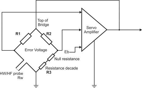
Most of the papers describe hot-wire anemometers using this diagram: |
 |
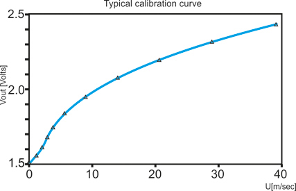 |
Fig. 1: Basic HWA circuit and a typical calibration curve of a 5 micron wire. |
The user is calibrating the wire by sampling few points at known velocities and a calibration curve is plotted. Sometimes, "King's law" is used for calibrations at high velocities.
However, this diagram describes maybe 10% of the components found in a commercial anemometer. Most of the commercial anemometers got plenty of other components used for improvement of the frequency response, automatic setup of parameters, protection circuits, various bridge ratios and cable compensation for the probe cable in one or more lengths.
|
The anemometer is a Non-linear system.
As one may see from the calibration graph, the CT Anemometer is a non-linear instrument. The voltage which is produced by this instrument is not a linear function of the velocity "input".
Therefore, the behavior of nonlinear systems is not subject to the principle of superposition while that of linear systems is subject to superposition. Thus, a complex nonlinear system is one whose behavior can't be expressed as a sum of the behaviors of its parts (or of their multiples). Fourier analysis use a sum of sine waves to describe periodic signals and they use the principle of superposition to test the response of each sine wave and according to that predict the response of a system according to the sum of the response curves to each sine wave - i.e. Fourier transforms/analysis and their features do not work on nonlinear systems!!!.
For example, you cannot do integration over the pulse response and get the step response like it is done in linear systems.
Features as static linearity and Sinusoidal fidelity do not exist in a non-linear system – If a sine wave is input in order to test the system's performance, the amplitude can be different – depending on the DC offset- and other frequencies (i.e. "harmonics") that would show at the output, although they did not exist in the input. Even if the non-linear system output is linearized, the whole system would still not have the sinusoidal fidelity. The reason for that is simple: We all know that the hot-wire anemometer calibration curve can be represented using a polynomial. No matter which degree is that polynomial, if we input a pure sine wave into a polynomial, we will get harmonics (which means different sine waves with different frequencies, amplitudes, phase – frequencies would be multiple of the original frequency). The higher the amplitude –more harmonics, at higher amplitudes would be present at the output. This is true for any non linear system and it can be checked in "Mat-Lab" or similar program using King's law and a synthetic sine wave or pulse or square wave.
Because of that "feature", linear operations as differentiation and integration cannot be used over a high amplitude signal in non-linear systems (maybe on a very small range assuming linear behavior in this region) for determining one system behavior from measurements of another one.
Most people think that due to the fact that the polynomial we use for CT Anemometer calibration is an Injective function, if we use an inverse polynomial for calibration, then after the inverse polynomial (usually found using Least Squares Fit method), we would get the same function as we originally had (which in our case means the same frequencies as were in the flow). This assumption was true if the CT anemometer was a mathematical function…
However, the CT anemometer is an electronic circuit with signal conditioner and low-pass filters. Each one of those frequencies created by the non-linear circuit has a different propagation delay. Some of the frequencies disappear due to the low bandwidth of the amplifier, Low pass filter (anti-aliasing filter) or the low sampling rate. When we sample them at the output, using an A2D converter, we get only the amplitude information. We actually lose the phase (or delay) information and then when we convert it back to velocity, using our LS fit polynomial, we get the original frequencies only for the low frequencies. Some of the high frequencies in the signal are added or subtracted from the same frequencies which were created from harmonics of lower frequencies and cannot be spread into their components. We also cannot reconstruct the high frequencies because they were phase shifted. Because of this non-linear phase shift, instead of "losing" the harmonics we got from the non-linear circuit, we gain more other harmonics. Because of that, measuring with a CTA at high frequencies is not 100% correct (and spectra graphs after calibration are worse).
|
Anemometer non-linearity effects on frequency response
As I explained above, the anemometer is a non-linear instrument and therefore standard mathematical tools used for analyzing linear systems do not work in this case.
The anemometer circuit reminds the classical "Mass-Damper-Spring" (MDS) frequency response. In both of them, the response is non-linear. The frequency response depends on the amplitude and the DC offset (or position in the MDS mechanical system). The following graph explains that behavior: |
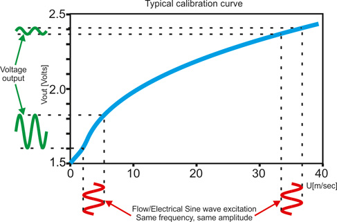 |
Fig 2: Sine wave excitation at the same amplitude, at different velocities, would yield a different output voltage.
|
This graph is actually describing something which is well known to any anemometer user: The sensitivity of the CTA system at low velocities is much higher than it is in high velocities (see the green sine wave on the left side).
If the same small amplitude sine wave is injected to such a system, the response would be dependent on the mean velocity when it was measured (i.e. the velocity offset). As we may see, if the sine wave was input at a low velocity (Red sine wave on the left side), then the amplitude of the output voltage (Green sine wave) would be much higher (lower Green sine wave) if the same sine wave excitation was input at a higher velocity. This explains the difference between spectra graphs which were taken at a different mean velocities although the anemometer adjustment was never changed and the probe is exactly the same! It is also very far from graphs obtained using a small amplitude electrical sine wave which should be taken at average flow speed at a laminar flow.
If the sine wave amplitude is much larger, then we would start to see that the shape of the output signal is not a sine wave any more. It would become a "stretched" sine wave (non-symmetrical) where the negative peaks are much different in their width and shape from the positive peaks.
The reason for that is harmonics which were added to the signal due to the non-linear nature of the system.
|
Can we use spectra graphs?
The spectra graph is obtained by mounting the probe in a turbulent flow (The HW probe is placed about 5-6 diameters from a jet, at the center).
A buffer of few tens of kilobytes is taken at a high sampling rate and the FFT is calculated (Real FFT with no imaginary component). The "Spectra" graph is an ensemble average over few tens of FFT plots (power spectrum) and then the "spectra" graph is obtained.The ensemble averaging remove noise and enhance only the parts of the FFT which were obtained in most of the FFT plots which were averaged.
The analog real time signal which we measure at a spectra graph looks like that: |
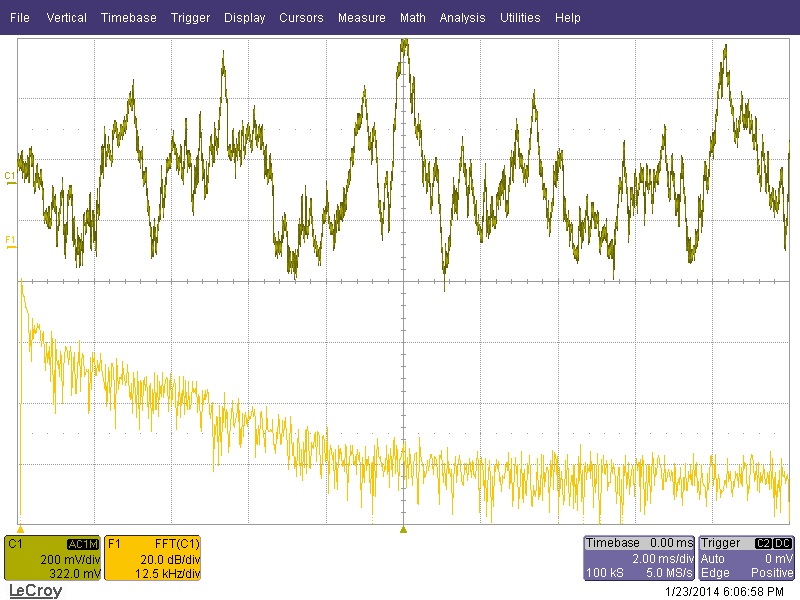 |
Fig. 3: an 8 bit oscilloscope screen shot of the turbulent signal at TOB (Green trace) and the FFT of this single screen shot (Yellow trace). This FFT is plotted using linear scales so it doesn't look the same as most log-log graphs shown in most papers.
|
Because of the non linearity, the "Spectra" tests of the CT anemometer are not so correct. When a spectra graph is taken (for example at 50m/sec) the voltage amplitude is about 1 Volt PTP at Top of the Bridge point (which corresponds to 0-50m/sec – see the calibration curve in Fig. 1)). As illustrated in Fig. 2, a high frequency sine wave which appears at low mean velocity would yield different amplitude from the same frequency and the same amplitude input at high mean velocity, due to the non-linear nature of the graph. Since the Spectra calibration is done BEFORE we linearize the bridge voltage (As explained above), it actually average frequency components with different amplitudes although they were created from similar flow amplitudes but at different flow "offsets". (In other words – a frequency component in some frequency "F" which exists at low velocity is averaged with the same frequency which present at high velocity. The spectra graph would show the average of the power of both signals). Because of that, the spectra graph is not so correct. As we may know, the shape of the spectra graph is also changed according to the maximum velocity, Overheat Ratio, Damping adjustment (i.e. pulse or square wave response), probe type, cable compensation adjustment and many other factors.
|
Damping adjustment influence the spectra:
We cannot determine exactly whether the power in some frequency "F" is the real energy in the flow or maybe due to wrong measurement or different adjustment of the bridge or harmonics which makes the power level looks higher than it is. The graphs in Fig. 4 below illustrate the spectra of a sensor in the same velocity (about 15 cm distances from a nozzle of 3cm diameter) at 50 m/sec. The graphs are taken from a Real-time spectra screen of our AN-1005 anemometer with the same channel module: |
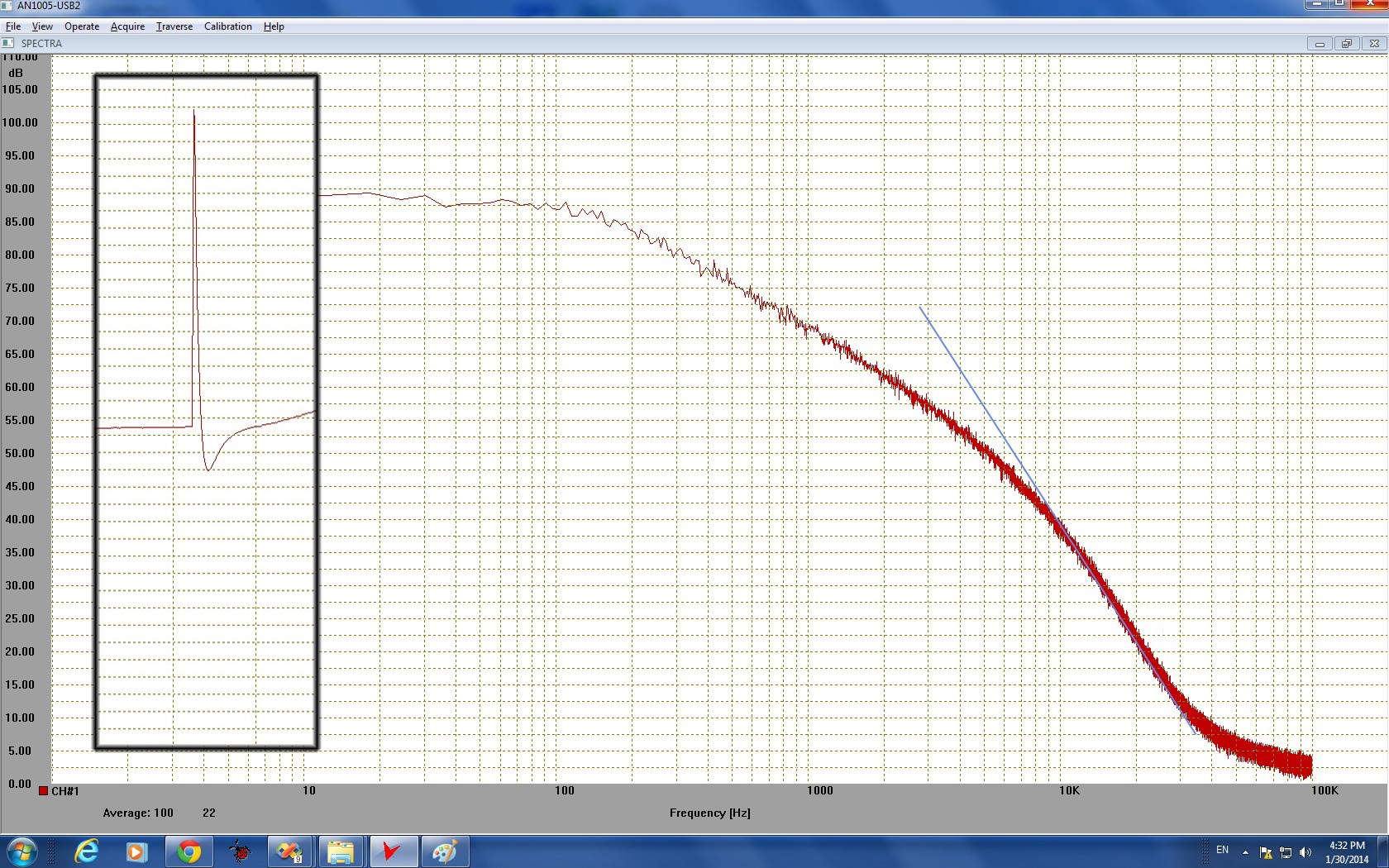 |
This spectra graph is attenuated at high frequencies (See the blue slope line that I plotted). The pulse response (on the left) is overdamped causing the slope of the decay to be lower (like a low-pass filter on the regular thermal response) |
 |
This spectra graph is attenuated at high frequencies (See the blue slope line that I plotted). The pulse response (on the left) is overdamped causing the slope of the decay to be lower (like a low-pass filter on the regular thermal response) |
|
|
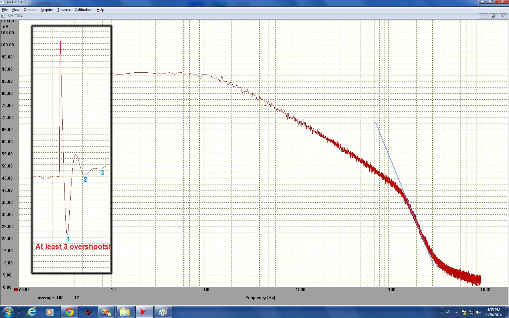
This graph is of an under-damped response.
As can be seen, there is a small resonance peak before the final roll-off. This setting is almost oscillating. The pulse response has many overshoots. |
| |
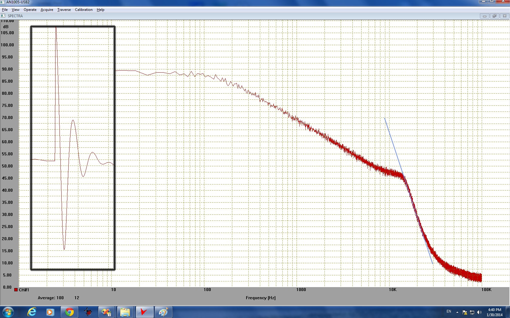
Fig. 4: 3 Real-Time Spectra graphs from AN-1005 software: The first plot is for over-damped response while the third plot is for under-damped response. As can be seen, the slope of the high frequency part of the spectra is changed by using the "Damping" adjustment only. Those graphs may look different for other overheat ratio, maximum velocity, different location of the HW sensor, different tuning of the cable compensation, different type of probe cable etc. On the left side of each plot I put the pulse response, in the same flow conditions where the spectra graphs were taken, with no filtering or signal processing of any kind (The pulse response graphs are not flat. There are some fluctuations from the turbulence on them).
|
Those graphs were taken from AN-1005 software which allows the user to see real-time spectra which refresh between few seconds to about 1.5 minute (Using Ensemble average of 10, 20, 50 or 100 FFT plots). The fast refresh rates allows the user to do adjustments using the "Damping" trimpot and the cable compensation and get the "right" shape which is suitable for their measurements.
Those graphs are AFTER signal conditioning. The bandwidth is far more than 100 KHz. This is the correct way of measuring the spectra because the user can select one of 12 built-in low pass filters found in the anemometer and limit the bandwidth (for Anti-Aliasing or noise reduction purpose). This is the final signal which goes to the A2D converter in every standard experiment – not the Top of Bridge signal like the authors of some papers used...
It can be seen on Fig. 7 that the spectra graph (when using a pulse test signal– not a square wave) looks like in theory when the damping settings of the pulse response is set to yield a pulse response with few overshoots (and the second and third overshoots are quite high). It has nothing to do with the adjustment suggested by the papers mentioned by the authors for anemometers which had a square wave test signal or in the paper written by P. Freymuth at 1977!. The conclusion from the graphs published by some authors (which shows a decayed response of AA Labs CT anemometer at high frequencies) is simple – the authors probably adjusted the AN-1003 system they had at maximum velocity using P. Freymuth's "thumb rule " for Square wave test signal – not with a Pulse test signal as it is (and without checking the adjustment instructions in the manual).
|
Cable compensation adjustment affects the spectra:
The cable compensation circuit (as called "high Frequency compensation") is used for balancing the capacitance and inductance on both arms of the bridge. It would work well only if a probe cable with low capacitance and inductance, as sold by the manufacturer, is used. If the customer is using a low quality cable (see our paper about selecting the probe cable) then the inductance and capacitance would be higher and the cable compensation would not work properly because the compensation circuit on the other arm of the bridge (inside the anemometer channel) would not have the same capacitance and inductance. On the following pictures we can see a fast spectra graph (only 20 averages) of the same channel with the same adjustment at the same flow. As we may see, on the right graph the cable is compensated much better so the -3dB point of the frequency response is about 35KHz. while on the left graph it is only about 18 Khz. The only difference between both graphs is different adjustments of the cable compensation circuit (option 04) + Damping trimpot. As you may see, the slope is the same, only higher bandwidth |
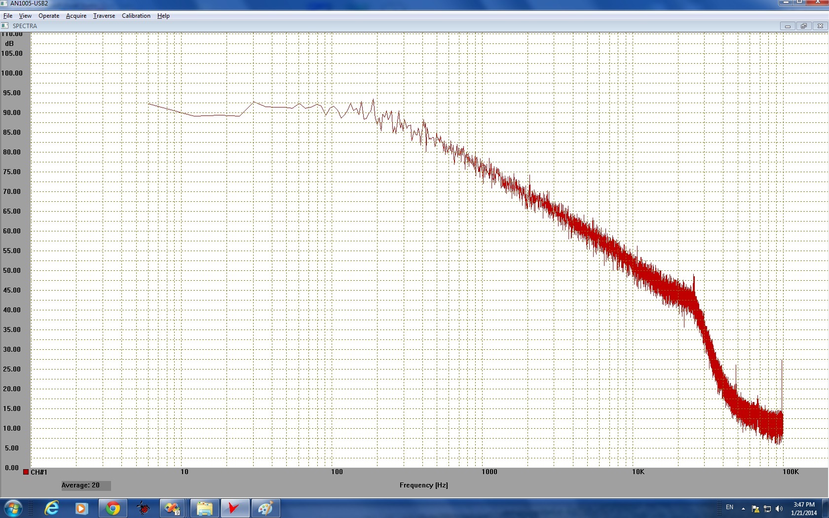 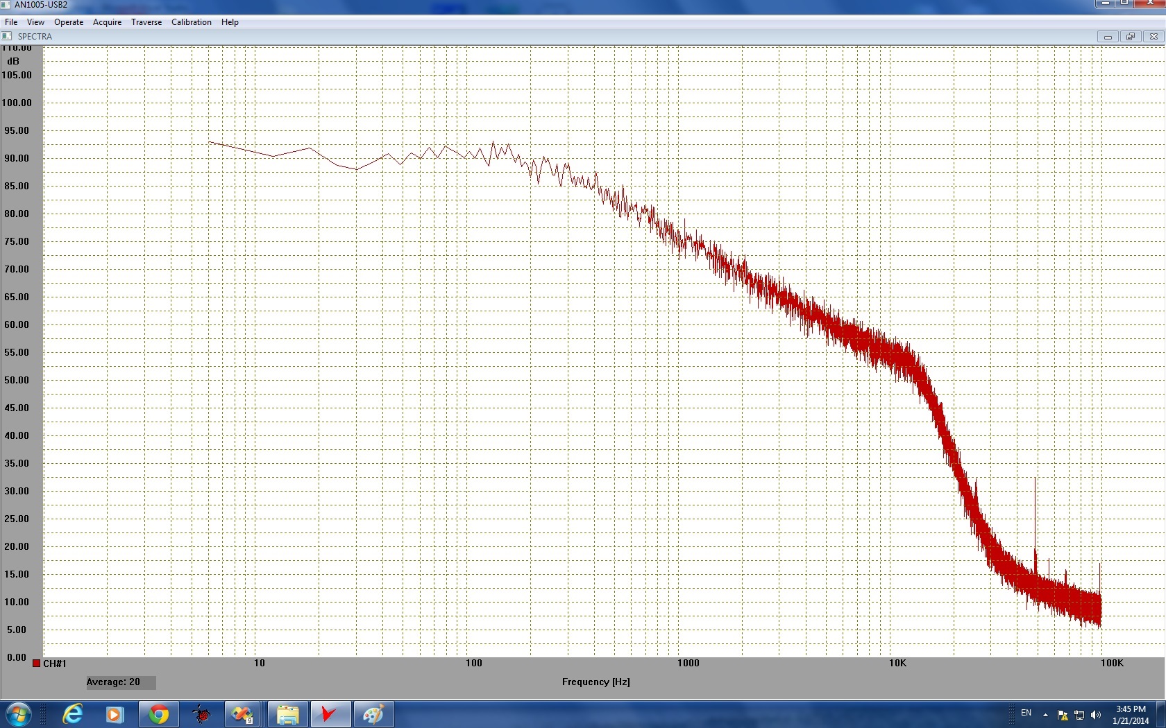 |
Figure 5: The influence of Option 04 on "Extending" the frequency response due to a better cable compensation. The graph is "thick" because we averaged only 20 FFT's. This is a real-time spectra screen from AN-1005 software.
|
Adjustments according to pulse/square wave response:
As we all know and read, many people quote Dr. Freymuth's paper:
"Frequency response and electronic testing of Hot Wire Anemometers" (1977).
He writes: "It is found that a well-designed anemometer behaves as a third order control system which allows for a two parameter optimization of its dynamic response". Fig. 4 in Dr. Freymuth's paper shows how the square wave response should look like. It is evident that in a "well-designed anemometer", the rise time and fall time of a square wave response should be almost the same and the response curve should be smooth. If the graph does not looks like that, then it is either not a square wave tested anemometer or maybe the anemometer is not "well designed" because the response is not a 3'rd order response.
Dr. Freymuth als suggests some "adjustment rules":
"The ‘optimum’ square-wave response is described by Freymuth (1977) as one in which there is a slight undershoot (of approximately 15% of the maximum)"
As will be shown in the examples later on this paper, those "recommendations" made by Dr. Freymuth, were true ONLY for a square wave test signal at some unknown amplitude which Dr. Freymuth was using. With all the respect to Dr. Freymuth, he did not bother to measure the amplitude, rise time and DC offset of his test signal. His "adjustment rules" are good only for the anemometer that he tested. His "thumb rule" of f = 1/1.3τ is good only for his experiment and for his setup. He probably "forgot" that the CT Anemometer is a non-linear system, which makes the step response to depend on those parameters of the test signal...
We claim that if we look for a general rule for setting anemometers and knowing their frequency response, then we cannot rely on "τ" which is the time of the rise and fall time immediately after the test signal was injected. This τ is test signal dependent parameter.
The following oscilloscope plots, taken on the same anemometer channels, with exactly the same probe, Overheat ratio, damping etc. explain why:
|
 |
 |
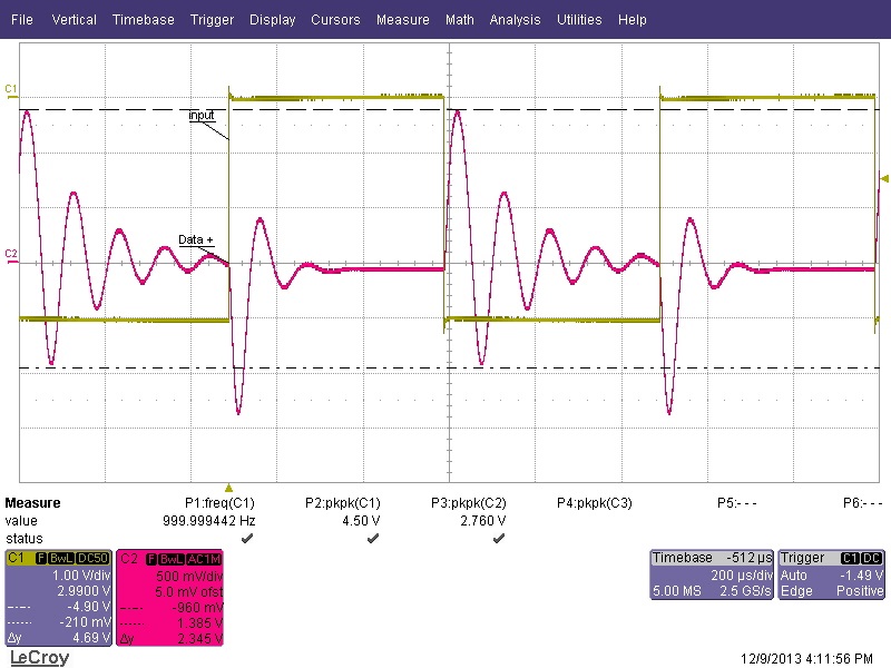 |
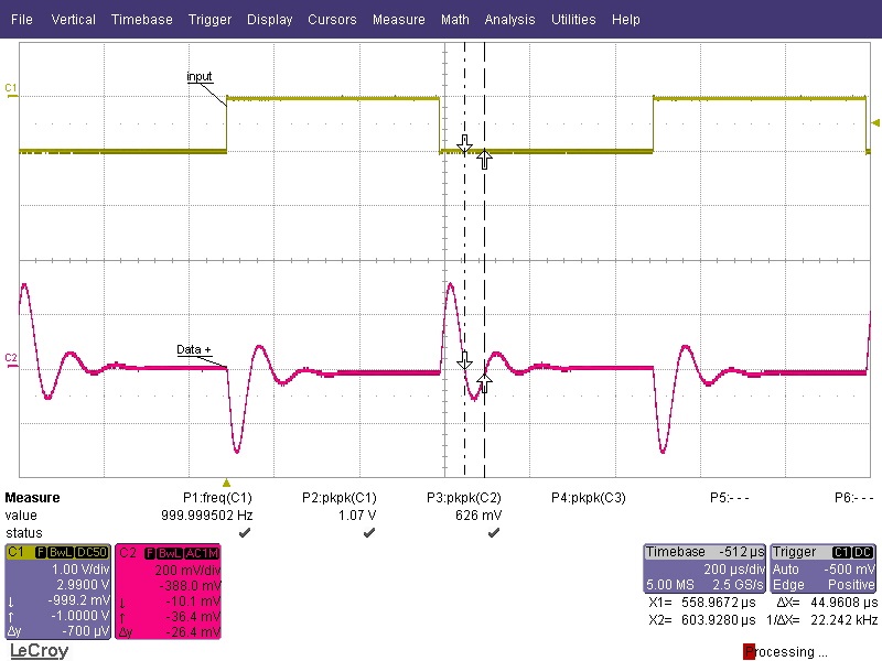
Fig 6: Square wave test of the same anemometer channel:
Left plot is using a standard low amplitude square wave. The response is similar on the rising and falling edge. The center plot is showing the same square wave shifted with some DC offset or different amplitude. In order to make those 3 plots an external function generator was used and only the "Amplitude", "DC offset" controls were used.
|
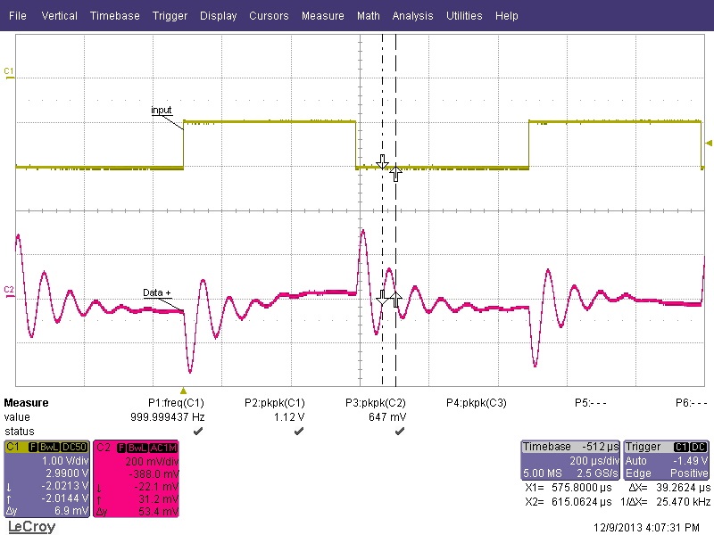
The response becomes different- The "τ" parameter is different between the 3 tests although we did not change anything in the anemometer or in the setup or in the flow! Just a different test signal! The right picture is showing the same anemometer with large scale test signal. As we may see, the response to the rising edge is absolutely different from the response to the falling edge! The "τ" is different. It is the exactly same in many other anemometers made by different brands, tested by us during the last 30 years. This example actually explains why does researchers argue during the last 37 years (Since P. Fremuth's paper on 1977) whether the frequency bandwidth (-3dB cut-off) can be estimated as f = 1/1.3 τ (Disa/Dantec systems) or f = 1/1.5 τ (TSI systems) or f = 1/1.6 τ Beljaars (1976) and Li (2004) – and there are at least 20 more papers which discuss that issue (as far as I know…).
As you may see, the same anemometer (which has the same spectra – nothing was changed!) can have 3 different response curves which depends only on the square wave amplitude and DC offset. Did any of those researchers mentioned what is the amplitude and DC offset of the square wave used to test their system? No!
Any anemometer manufacturer cannot "tune" the pulse or square wave input to have the same amplitude, DC offset and rise time in all of anemometers that they manufacture! In our anemometers, the amplitude of the pulse (or the frequency and duty cycle in our AN-1005 system) can be adjusted by the user, so the adjustment of the pulse response is actually dependent on what the user adjusted and nothing else!
As we can see in Fig. 6 above, the τ of the 3 response plots is different due to the different test signal.
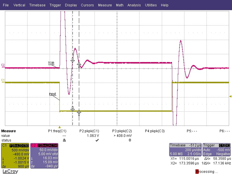
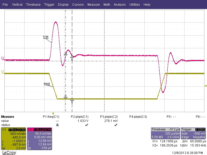
The same problem exists if the rise time of the square wave test signal is not the same. In the 3 plots below we see a response to a high amplitude square wave compared to an exaggerated low rise time square wave response to a square wave response with a high rise time. All response curves were taken from the same anemometer with the same probe and the same adjustments:
|
 |
 |
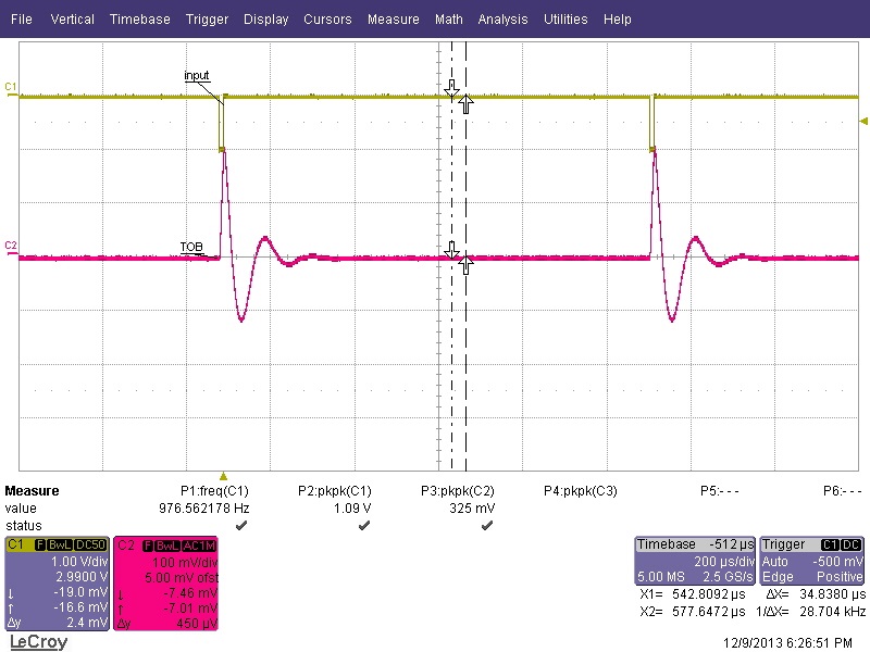 |
Fig. 7: Three different response shapes and different "τ" for the same anemometer channel module, using the same probe, same cable and the same setup. The oscilloscope is adjusted to the same time base on all 3 pictures. In order to make those 3 plots an external function generator was used and only the "Duty Cycle", "rise time" and "Fall Time" controls were used. The anemometer, probe, flow velocity, OHR, damping setting and all other parameters are the same as in Fig. 6 above.
Those are actual JPG screenshots taken from a State-of-the-art "LECROY" oscilloscope. They were not "Ensemble averaged" or "High Pass filtered" or "simple threshold techniques" were used (as some researchers do) or edited or altered in any way.
|
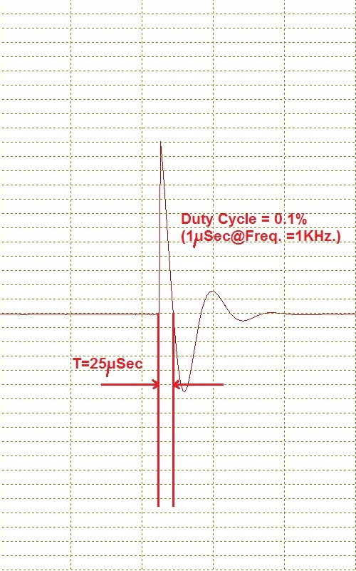
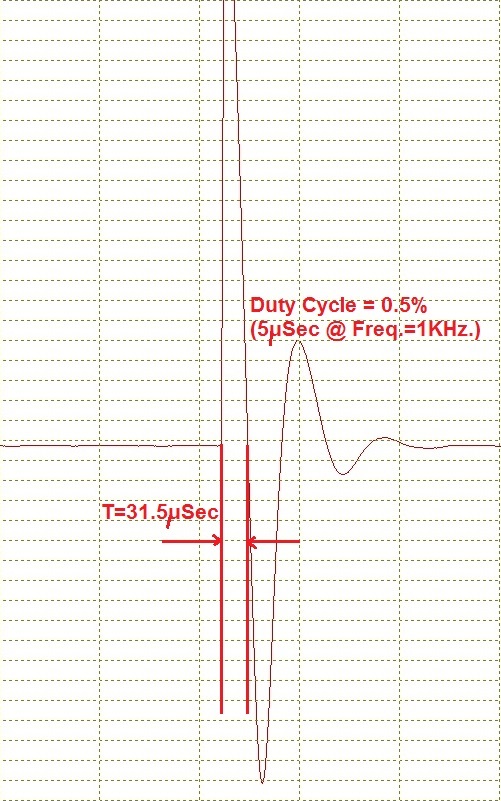
In our AN-1005 Anemometer, the excitation signal is a pulse and the width of the pulse can be changed: |
 |
 |
|
Fig 8: Different τ in pulse response due to a different pulse width test signal. All other Anemometer adjustments are exactly the same.
|
As can be seen in all above examples, the "τ" measured by Dr. Freymuth is different depending on the DC offset, Amplitude, rise time, Fall Time and pulse width of the test signal input. Any "Comparisons" between one anemometer to another (even from the same model, made by the same manufacturer) are wrong and have no scientific value! In addition to that, the pulse is injected thru a resistor which is absolutely different from one model to another (usually because the internal test generator is different). Therefore, input of the same square wave or pulse to different model would yield different results! This is a non-linear system! Look again at Fig. 2 above and you would understand why!
If you would like to make sure that those conclusions are good for any second or 3'rd order system, please use any 2'nd or 3'rd order system model found in Mat-Lab and use synthetic signals to test them. The conclusions would be the same!
If the amplitude is changed or the gain/resistance of the test signal is changed, then all of this "Thumb rule" worth nothing because the user may over-damp (if the test signal is too strong) or under-damp (if the test signal is too weak) the square wave response while causing the system to be over-damped or under-damped and still have the same shape of the square wave response on all of the tests/Anemometers.
|
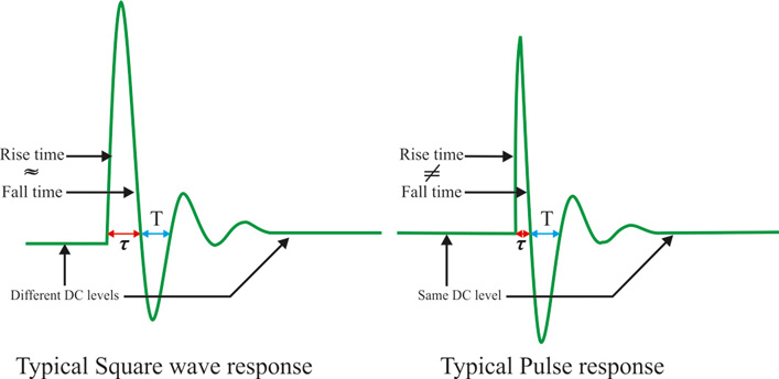 |
Fig. 9: The difference between a square wave response to a pulse response – in any anemometer – no matter who makes it.
|
It is evident, in all above pictures and examples that " τ " is test signal dependent while T is not. In all examples above, T represent the natural frequency of the systems and it is almost the same, no matter which test signal is used.
As we may see, other scientists also disagree with Dr. Freymuth:
Freymuth claims a ratio of f = 1/1.3 τ.
On another paper, issued by another big manufacturer of HWA systems and probes from USA we can read that "A very fine HW probe by itself cannot respond to changes in velocity at freq. above 500 Hz." And "with electronic compensation….can be increased to 300-500 KHz." (This text was copied from a manual of an anemometer which was used on those days in the 70's when Freymuth wrote his paper).
We also read there that" f = 1/1.5 τ = The frequency in Hz at which closed loop response is attenuated by -3dB" (or in other words, the -3dB point is at that frequency). However, on this anemometer, manufactured over 38 years ago, the ratio was 1.5 and not 1.3 as in the system made by the other manufacturer.
Beljaars (1976) suggested that the attenuation effect starts at 2πfl =ωl ≈ 10/ τ. This ratio has also been confirmed in Li (at 2004).
Using those results, we can do a fast calculation and find that fl = 10/2πτ or in other words,
fl = 10/2π τ = 1/1.6 τ!!! So now the "Magic number" is probably 1.6! Not 1.3 or 1.5 as other researchers claimed...
There are tens of other examples in the literature, starting from a ratio of 1.2 and ending at a ratio of 1.8!!! At none of those papers the authors mention the damping setting (i.e. control voltage used and its amplification factor), the cable type and its length and the exact shape of the test signal – duty cycle, rise time, fall time and amplitude. I wonder why did they waste so much energy on those papers over the last 40 years without doing those simple measurements. How can those results be repeated by other researchers which do not have an identical anemometer? (Even 2 anemometer models made by the same manufacturer do not have an identical test signal and not an identical response…)
There are no scientific benefits from all of those comparisons and papers because every anemometer is designed in a different way and tested at different conditions! Every test input has a different gain, as explained above! And the users adjust it differently!
The conclusion is simple:
The square wave/pulse test is good only for first adjustment in order to keep the anemometer stable with no oscillations.
The "Tau thumb rule" is a test signal dependent and anemometer dependent rule. It is obviously not a physics law or empirical law, even if it was claimed in a paper made by P. Freymuth (at 1977) which was one of the leading researchers in HWA. With all the respect, he used one particular anemometer made by one company and did not compare to the other systems and did not do the same measurement with different types of probes, cables and settings of "damping factor" and "HF filters".
I can sadly say that some researchers show odd graphs where their data was probably edited just in order to "fit" them to one thumb rule or another:
I will not mention those researchers name but I can just say that they have some connection to a new "one man" company who makes anemometers…
Here is our drawing showing a square wave test of their anemometer (this is the "artist impression" of their graph – we did not get their permission to put the actual graph):
Such a response is not a 3'rd order response. A 3'rd order response of a system with such a low natural frequency cannot change its slope 3 times within less than a single microsecond… |
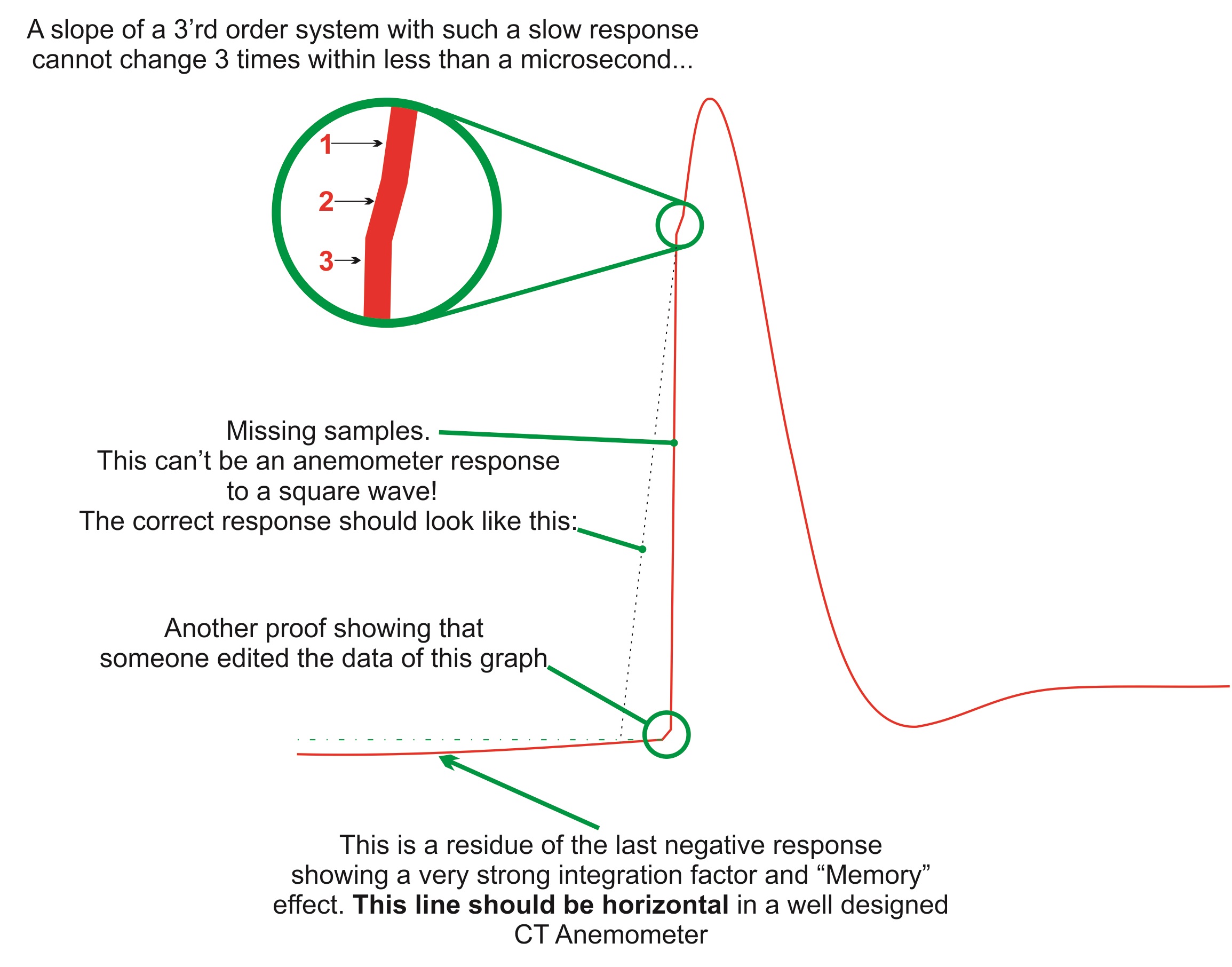 |
Fig. 10: A square wave response of a "homemade" anemometer published by one of the research groups. Comments are inside the picture.
(The graph on the left is an "artist impression" of actual zooming of one of the graphs they published – see above).
|
As you may know, a "well designed anemometer" is a 3'rd order system (P. Freymuth, 1977). This is definitely not a response of a 3'rd order system!
So the question is whether this is the real response or the poor researcher simply cut some data points in order to comply with P. Freymuth's thumb rules?
The conclusions from this article are simple:
Use the pulse response in your anemometer only in order to make sure that the circuit is stable.
In a square wave tested anemometer you might need 1-2 overshoots where the first one is at least 15%-25% of the first positive rising edge of the response curve in order to make a stable adjustment. In a pulse driven anemometer – you need to adjust to 2-3 overshoots in order to get the same spectra adjustment. Those adjustments must be done in average flow speed.
When you use a thumb rule f = 1/1.3 τ or f = 1/1.6 τ… use the time T instead of the time τ. T is not test signal dependent. We can't tell whether the factor is 1.3 or 1.6 because we observed both cases with our anemometers using different probes, different Overheat Ratio values and different settings.
In our anemometers you may adjust the amplitude of the pulse and in AN-1005 you may adjust the pulse width so th "T" or "Tau" would fit thte "thumb rule" you are used to. It is the responsibility of the user to adjust it so the -3dB point will comply with the "thumb rule" he is used to. Always do a spectra graph later, to verify that at high frequencies the response is as you wish to have (unless you don't work at high frequencies).
According to our experience, the cable compensation adjustment (Option 04) is also important to having a higher frequency response. Bad adjustment of Option 04 screw may cause odd results and change the shape of your spectra! This adjustment must be done together with the "Damping" trimpot. Otherwise, you will get very strange spectra as some researchers got…
Can different anemometers be compared?
Sometimes we see papers where researchers try to compare between anemometers using their internal test signals or sometimes by using an external test signal as a Sine wave. All of those comparisons are wrong and have nothing to do with the reality. There are several reasons for that:
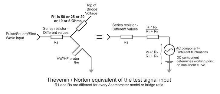
1. Different test signal – Some anemometers are tested by pulse, some by square wave. As explained above, the Amplitude, Duty Cycle, Rise and Fall times, DC offset of the test signal change the results. In addition to that, every anemometer got a different series resistor connected between the bridge to the test generator (or BNC). This means that the gain of the input signal is not the same.
In
addition to that, the bridge ratio might not be the same and also the top resistance (the resistance between the output of the servo amplifier – Top of Bridge – to the sensor) is different. On some anemometers it is 10 or 20 ohms, on some others it is 25 or 50 Ohms and we have already modified some of our anemometers to have 500 or 1000 ohms in series as well as 5 or 10 Ohms in series for custom made sensors.
2. The junction of the probe and the top resistance mentioned above is connected to the series resistor which comes from the test generator. Beside the fact that it applies a different load on the test signal (Thévenin and Norton Theorem) thus the test signal would have a different Voltage/current gain for every probe resistance or Top resistance, It also change the DC offset of the test signal (because the junction mentioned above is summing the voltage coming from a voltage divider of the sensor + top resistance and from the test signal coming thru the series resistance. We have already discussed above in details the effect of DC offset and Amplitude/ different gain of the test signal on the response.
The best proof of that is when the bridge ratio is switched (on any anemometer), the response is not the same any more although it it the same anemometer with the same servo amplifier.
3. The same thing is true with a Sine wave test. This tool is good for testing the frequency response of the anemometer (i.e. flatness, slope etc). However, the results of this test does not always comply with the Spectra test because some manufacturers use internal HF filters to increase the electrical response of their Anemometes. When not adjusted correctly, it might yield odd results like resonance before the -3dB point or even after it! Those filters also change the sine wave test response. We don't put such HF filters in our systems because they cause more damage than help. They increase the noise tramendously and it is very difficult to adjust them because there are only few filters. THey do not match exactly the response of every sensor, in every Overheat Ratio, In every damping adjustment. There would always be a small "hole" or "bump" in the spectra when those HF filters are used.
Maybe 20 years ago a skilled user could spend few hours and tune teh response with those filters to extend the frequency bandwidth of his anemometer without having "bumps" in his spectra graph. However, today, when fast computers are available, Those filters are useless and it can easily done using software filters found in any mathematical or signal processing program.
It is the same idea like "Conditional sampling" which was used 20 or 30 years ago when the bigggest hard drive available was 10 MB... Who needs that today when a 2 TB hard drive cost less than $100?
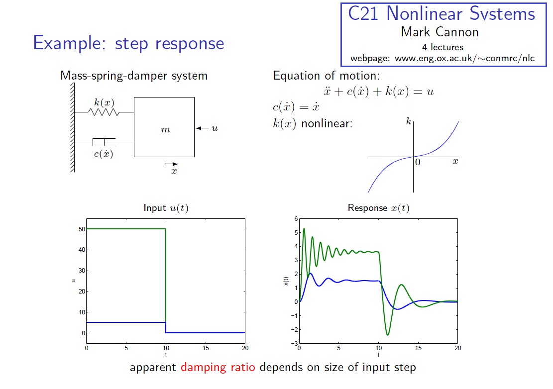
Another interesting example is from the mechanics world - A Mass-Spring Damper system. Although it is a second order system and not a 3'rd order system as the CTA anemometer, it behaves quite the same.
Here is a nice slide taken from a course in Nonlinear systems by Mark Cannon from university of Oxford, UK: |
(click on the image to see original lecture) |
As can be seen, the output amplitude is nonlinear with the input. The input step is increased by a factor of 10 and the output change by a factor of 2 only. The step input and it's response are plotted with the same color. When a higher amplitude step is input to this system, not only the amplitude would change - also the time "τ" is changing... The damping is also dependent on the amplitude of the test signal (the input step). Very similar to the CT Anemometer...
|
The best tool for getting a flat response is using a spectra graph. Although it is not 100% accurate (because a sine wave flow signal, even if it has the same amplitude, would show different output voltage (Peak to peak) if it is "riding" on low velocity or if it is riding over a high velocity (see fig. 2 above) - It would still allow the user to have a good "Flat" statistical tool for having a fast view of the spectra and use the "Damping" control and cable compensation to tune it in real time. It is also recommended to use this tool for finding turbulence in any flow. It is most recommended to use it in fast mode (like 20 ensemble averages of the FFT plots) for the first adjustment and a slow mode (about 100-200 plots averaged) for fine tuning (slower refresh times).
If you like to increase your frequency response over the natural thermal response of the probe + anemometer, we highly recommend using a software algorithm that would "fix" the spectra:
|
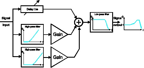 |
Such an algorithm can be implemented only using anemometers with very low noise like our anemometers with Option 01.
It cannot be used with anemometers with over 1-2mV ptp noise at top of the bridge because the noise is also amplified and it would destroy the resolution of the signal and would not allow resolving low level turbulence. |
| |
Avi Aharoni
A. A. Lab Systems |